A trigonometrikus és hiperbolikus függvények, illetve ezek inverzei
A hiperbolikus függvények a matematikában a szögfüggvényekhez hasonló függvények.
A két alapvető hiperbolikus függvény a hiperbolikus szinusz (jelölése sh vagy sinh) és a hiperbolikus koszinusz (jelölése ch vagy cosh), melyekből levezethető a hiperbolikus tangens (jelölése th vagy tanh) függvény a szögfüggvényekhez hasonlóan. Ugyanúgy számolható belőlük a hiperbolikus szekáns és a hiperbolikus koszekáns, mint trigonometrikus megfelelőikből a szekáns és a koszekáns. Ezeknek a függvényeknek az inverzei az area hiperbolikus függvények. Ezt az adott függvény neve elé tett area szó jelzi. Mindezek a függvények egyes szerzőknél latin nevükkel szerepelnek, mint sinus hyperbolicus, cosinus hyperbolicus, tangens hyperbolicus, cotangens hyperbolicus, secans hyperbolicus, cosecans hyperbolicus; illetve az area függvények: area sinus hyperbolicus, area cosinus hyperbolicus, area tangens hyperbolicus, area cotangens hyperbolicus, area secans hyperbolicus, area cosecans hyperbolicus.
Ahogy a (cos t, sin t) pontok egy kört határoznak meg, az az egységkört, úgy a (ch t, sh t) pontok egy hiperbola jobb oldali félgörbéjét írják le, mely az egységhiperbolához tartozik. A kapcsolat a komplex számsíkon még nyilvánvalóbb, mivel . Így például . A komplex hiperbolikus szinusz és hiperbolikus koszinusz az egész komplex számsíkon folytonosan definiált, sőt holomorf függvények. A többi hiperbolikus függvénynek pólusai vannak a képzetes tengelyen.
A hiperbolikus függvények azért is fontosak, mert több lineáris differenciálegyenlet megoldását fel lehet írni a használatukkal. Ilyen például derékszögű koordináta-rendszerben a súlya alatt lelógó kábel egyenlete. Alkalmazhatóak ezen kívül a Laplace-egyenlet megoldásánál, amely a fizika több területén – az elektromágnesség elméletében, hőátadásban, folyadékok dinamikájában és a speciális relativitáselméletben – is fontos.
Definíciók
Az origóbóél kiinduló sugár az hiperbolát az pontban metszi, ahol a sugár, az -tengelyre vett tükörképe és a hiperbola által közrezárt terület
Az egységhiperbola egyenlete , így a két alapvető hiperbolikus függvény, a hiperbolikus koszinusz és a hiperbolikus szinusz:
Hasonló kapcsolatban állnak, mint a trigonometrikus függvények az egységkörrel:
Itt az egyenes és a hiperbola metszéspontjának koordinátája, és az egyenes és a hiperbola metszéspontjának koordinátája. A értéke az koordináta az helyen, azaz az egyenes meredeksége.
Ha a területet integrálással számítjuk ki, akkor az exponenciális ábrázoláshoz jutunk, ami használható ekvivalens definícióként:
Ez alapján a hatványsorok:
Itt az szám faktoriálisa, vagyis az első pozitív egész szám szorzata. Szemben a és a hatványsorával, itt nincsenek negatív együtthatók.
Tulajdonságok
sh és ch
Minden valós számra és valós.
A valós függvény értékkészlete az összes valós szám; a valós értékkészletébe az egynél nem kisebb valós számok tartoznak.
A valós függvény szigorúan monoton nő, és a nulla helyen inflexiós pontja van, ahol nullhelye is van.
A valós szigorúan monoton csökken az intervallumon, és szigorúan monoton nő az intervallumon. Globális minimumát az helyen éri el.
A valós függvény aszimptotikus függvényei és . A valós függvény aszimptotikus függvényei és .
Mivel , azért a komplex hiperbolikus függvénytulajdonságok a valós függvényekre is teljesülnek:
Az függvény páratlan, az függvény páros.
A függvények periodikusak, periódusuk . Ez a valós függvényeken nem látszik, mivel a periódus tisztán képzetes; tehát a valós függvények nem periodikusak.
A következő szakaszok további összefüggéseket mutatnak be.
th és cth
Minden valós számra és minden nullától különböző valós számra valós. A függvény nem értelmezett nullában, ahol pólusa van.
A valós értékkészlete , a valós függvényé .
A valós függvénynek az helyen nullhelye van, ami inflexiós pont is.
A valós függvény szigorúan monoton nő; szigorúan monoton csökken, ha , és szigorúan monoton csökken, ha
Nem periodikus, páratlan függvények.
A valós aszimptotikus függvényei és . A valós függvény aszimptotikus függvényei és
sech és csch
Minden valós számra és minden nullától különböző valós számra valós. A függvény nem értelmezett nullában, ahol pólusa van.
A valós függvény értékkészlete ; a valós függvényé .
A valós függvény szigorúan monoton nő, ha , és szigorúan monoton csökken, ha . A valós függvény szigorúan monoton csökken, ha , és szigorúan monoton csökken, ha .
Nem periodikusak. páros, páratlan.
Mindkét függvénynek aszimptotája , ha .
A valós függvény maximumát az pontban éri el. a valós függvénynek nincsenek szélsőértékei.
A valós függvény inflexiós pontja az helyen vannak. A valós függvénynek nincsenek inflexiós pontjai.
lineáris differenciálegyenlet alaprendszerét, más néven megoldásbázisát alkotják, ugyanúgy mint az és függvények. Ha a két függvény számára kezdeti feltételként előírjuk, hogy , és , legyen, akkor ezzel a és függvényeket választottuk. Ezeket a tulajdonságokat a definícióból is bizonyítani lehet.
A függvény megoldja a következő differenciálegyenleteket
áreaszinusz hiperbolikus és áreakoszinusz hiperbolikus
áreatangens hiperbolikus és áreakotangens hiperbolikus
áreaszekáns hiperbolikus és áreakoszekáns hiperbolikus
Az inverz függvényeket csak olyan leszűkítéseken lehet definiálni, ahol az adott függvény egyértelmű. Így a szinusz hiperbolikust nem kell leszűkíteni, de például a koszinusz hiperbolikust igen: a koszinusz hipőerbolikust az korlátozva definiálják az área koszinusz hiperbolikust. Elemi módszerekkel kiszámolható, hogy:
.
.
A tangens hiperbolicus bijektív függvény. Inverz függvénye az area tangens hiperbolicus, ami az intervallumon értelmezett:
Az area cotangens hiperbolicus:
a intervallumon kívül értelmezve.
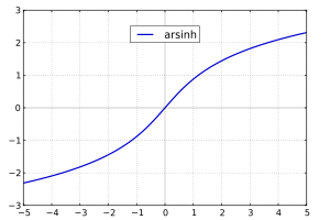
Az áreafüggvények grafikonja
áreaszinusz hiperbolikus
áreakoszinusz hiperbolikus
áreatangens hiperbolikus
áreakotangens hiperbolikus
áreaszekáns hiperbolikus
áreakoszekáns hiperbolikus
Hasonlóságok a szögfüggvényekkel
Kör és hiperbola kapcsolata
Az x y = 1 hiperbola x > 1 tartományban lévő tetszőleges pontja hiperbolikus háromszöget határoz meg, amelyben a hiperbolikus szög melletti oldal a ch értékkel egyenlő, míg a szöggel szemben fekvő oldal az sh-val. Azonban mivel a hiperbola (1,1) pontja az origótól √2 távolságra van, ezért az oldalak hosszát 1/√2 tényezővel kell szoroznunk, hogy a helyes eredményt kapjuk.
Mint ahogy a (cos x, sin x) pontok egy kört ( x2 + y2 = 1) határoznak meg, a (ch x, sh x) pontok az x² - y² = 1 egyenlő szárú hiperbola jobb oldali görbéjét írják le. Ez ezen a könnyen ellenőrizhető azonosságon:
és azon alapul, hogy ch x > 0 minden x-re.
A hiperbolikus függvények periodikusak komplex periódus szerint.
A x paraméter nem a kör középponti szöge, mint a szögfüggvényeknél, hanem a hiperbolikus „szög”, amelynek értéke a kétszerese annak a területnek, melyet az x tengely, a hiperbola és egy, a hiperbola (ch x, sh x) pontjából az origóba húzott egyenes határol.
A hiperbolikus függvényekre igen sok olyan azonosság érvényes, melyek hasonlóak a szögfüggvények azonosságaihoz. Az Osborne-szabály kimondja, hogy minden trigonometrikus azonosságot egy analóg hiperbolikus azonossággá lehet alakítani a következőképpen:
lecseréljük a szögfüggvényt a hiperbolikus megfelelőjével és
az sh * sh kifejezés előjelét megváltoztatjuk.
Néhány példa:
A „kétszeres szög” képletek:
és a „fél-szög” képletek:
Megjegyzés: Ez megfelel a szögfüggvény párjának.
Megjegyzés: Ez megfelel a szögfüggvény párja szorozva (-1)-gyel.
A tangens hyperbolicus számítható a képlettel. Ez azonban nagy, illetve kis abszolútértékű helyeken gondot okoz:
Nagy értékeknél túlcsordulás jön létre, habár az eredmény nagysága ezt nem indokolja
Kis értékek esetén vészes kiegyszerűsödés adódik, így az eredmény pontatlan lesz.
Ekkor a következő közelítések alkalmazhatók:
akkora pozitív szám, hogy . Ekkor
, ahol a szignifikáns számjegyek száma az adott számtípusnál, például double esetén 16.
nagy abszolútértékű negatív szám úgy, hogy , ahol szerepe a nagy pozitív számnál szereplő -hoz hasonló. Ekkor az előző esethez hasonlóan .
abszolútértékben kicsi. Például, ha , akkor ,
ahol jól közelíthető Taylor-sorának első néhány tagjával:
A többi hely esetén marad az eredeti képlet:
Alkalmazások
Az differenciálegyenlet megoldásai az
, ahol
alakú függvények.
Egy csak saját súlya által terhelt homogén lánc alakját hiperbolikus koszinusz függvénnyel lehet leírni. Ezt az alakot láncgörbének vagy katenoidnak hívják.
Egy x irányú Lorentz-transzformáció rapiditása segítségével a transzformáció mátrixa így írható le:
Látható a hasonlóság a forgatómátrixszal, amivel a négydimenziós Lorentz-transzformációk és a forgatások közötti hasonlóság is felismerhető.
A hiperbolikus szinusz és koszinusz a kozmológiában is előfordul. Egy lapos univerzumban, mely lényegében csak anyagot és sötét energiát tartalmaz (és ezáltal a mi univerzumunk közelítése), a skálafaktorok növekedését leíró összefüggés:
,
ahol karakterisztikus időskála; aktuális Hubble-paraméter és a sötét energia sűrűségparamétere. Az anyag sűrűségparaméterének időbeli függőségénél a koszinusz hiperbolikusz bukkan fel:
.
A tangens és a cotangens hyperbolicus használható arra, hogy az eltelt idő függvényében kiszámítsuk a légellenállásos esés sebességét, illetve turbulens áramlásban esik a tárgy (Newton-súrlódás). A koordináta-rendszert úgy rögzítjük, hogy a helytengely felfelé mutasson, tehát a térbeli mozgás tükörképeként. A sebesség az differenciálegyenletből számítható, ahol nehézségi gyorsulás, pozitív konstans, melynek mértékegysége . A végsebesség , ami a sebesség határértéke. Teljesül továbbá, hogy:
az esés vagy hajítás kezdeti sebessége kisebb, mint a végsebesség: , ahol
hajítás esetén a kezdősebesség nagyobb, mint a végsebesség: , ahol
A speciális relativitáselméletben a sebesség és a rapiditás összefüggése , ahol a fénysebesség.
A kvantummechanikában egy kétállapotú rendszert ért termikus hatást írja le: Legyen az állapotokat ért összhatás, és az állapotok közötti energiakülönbség. Így a hatásszámok különbsége , ahol Boltzmann-állandó, és abszolút hőmérséklet.
Paramágnes mágnesesezésének leírásához fontos a Brillouin-függvény:
A kozmológiában Egy lapos univerzumban, mely lényegében csak anyagot és sötét energiát tartalmaz (és ezáltal a mi univerzumunk közelítése), a Hubble-paraméter időbeli változását leíró összefüggés: , ahol karakterisztikus időskála, és a Hubble-paraméter határértéke esetén; a Hubble-paraméter kiinduláskori értéke, és a sötét energia sűrűségparamétere. A sötét energia sűrűségparaméterét pedig az . összefüggés írja le.
GonioLab: Egységsugarú kör, szögfüggvények és hiperbolikus függvények szemléltetése.
Források
Ilja N. Bronstein: Taschenbuch der Mathematik. Deutsch (Harri).
Yu. V. Sudorov. Inverse hyperbolic functions
Fordítás
Ez a szócikk részben vagy egészben a Hyperbelfunktion című német Wikipédia-szócikk fordításán alapul. Az eredeti cikk szerkesztőit annak laptörténete sorolja fel. Ez a jelzés csupán a megfogalmazás eredetét és a szerzői jogokat jelzi, nem szolgál a cikkben szereplő információk forrásmegjelöléseként.
Ez a szócikk részben vagy egészben az Areafunktion című német Wikipédia-szócikk fordításán alapul. Az eredeti cikk szerkesztőit annak laptörténete sorolja fel. Ez a jelzés csupán a megfogalmazás eredetét és a szerzői jogokat jelzi, nem szolgál a cikkben szereplő információk forrásmegjelöléseként.
Ez a szócikk részben vagy egészben a Sinus hyperbolicus und Kosinus hyperbolicus című német Wikipédia-szócikk fordításán alapul. Az eredeti cikk szerkesztőit annak laptörténete sorolja fel. Ez a jelzés csupán a megfogalmazás eredetét és a szerzői jogokat jelzi, nem szolgál a cikkben szereplő információk forrásmegjelöléseként.
Ez a szócikk részben vagy egészben a Tangens hyperbolicus und Kotangens hyperbolicus című német Wikipédia-szócikk fordításán alapul. Az eredeti cikk szerkesztőit annak laptörténete sorolja fel. Ez a jelzés csupán a megfogalmazás eredetét és a szerzői jogokat jelzi, nem szolgál a cikkben szereplő információk forrásmegjelöléseként.
Ez a szócikk részben vagy egészben a Sekans hyperbolicus und Kosekans hyperbolicus című német Wikipédia-szócikk fordításán alapul. Az eredeti cikk szerkesztőit annak laptörténete sorolja fel. Ez a jelzés csupán a megfogalmazás eredetét és a szerzői jogokat jelzi, nem szolgál a cikkben szereplő információk forrásmegjelöléseként.


![{\displaystyle (-\infty ,0]}](https://wikimedia.org/api/rest_v1/media/math/render/svg/0241c015ef4c611c9c9aeafb395e7c4a16178405)


![{\displaystyle \operatorname {th} x=\operatorname {sgn} x\left[1+\sum \limits _{k=1}^{\infty }(-1)^{k}\,2\,\mathrm {e} ^{-2k|x|}\right]}](https://wikimedia.org/api/rest_v1/media/math/render/svg/d95654584ab6d1b4f69a2fdf0c961723d100461e)


 áreaszinusz hiperbolikus
 áreakoszinusz hiperbolikus
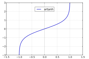 áreatangens hiperbolikus
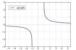 áreakotangens hiperbolikus
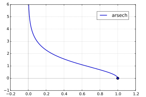 áreaszekáns hiperbolikus
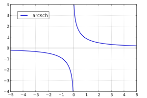 áreakoszekáns hiperbolikus


![{\displaystyle B_{J}(x)={\frac {1}{J}}\left[\left(J+{\frac {1}{2}}\right)\operatorname {cth} \left(J\,x+{\frac {x}{2}}\right)-{\frac {1}{2}}\operatorname {cth} {\frac {x}{2}}\right]}](https://wikimedia.org/api/rest_v1/media/math/render/svg/1ead61c782100c07af4648dd87309dcf09b344de)


