Elliptic coordinate system

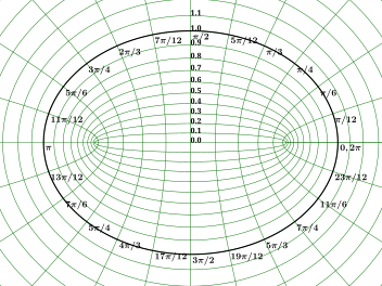
2D coordinate system whose coordinate lines are confocal ellipses and hyperbolae
Elliptic coordinate system

In geometry, the elliptic coordinate system is a two-dimensional orthogonal coordinate system in which the coordinate lines are confocal ellipses and hyperbolae. The two foci F 1 {\displaystyle F_{1}} and F 2 {\displaystyle F_{2}} are generally taken to be fixed at a {\displaystyle -a} and + a {\displaystyle +a} , respectively, on the x {\displaystyle x} -axis of the Cartesian coordinate system.

Basic definition

The most common definition of elliptic coordinates ( μ , ν ) {\displaystyle (\mu ,\nu )} is

x = a   cosh μ   cos ν y = a   sinh μ   sin ν {\displaystyle {\begin{aligned}x&=a\ \cosh \mu \ \cos \nu \\y&=a\ \sinh \mu \ \sin \nu \end{aligned}}}

where μ {\displaystyle \mu } is a nonnegative real number and ν [ 0 , 2 π ] . {\displaystyle \nu \in [0,2\pi ].}

On the complex plane, an equivalent relationship is

x + i y = a   cosh ( μ + i ν ) {\displaystyle x+iy=a\ \cosh(\mu +i\nu )}

These definitions correspond to ellipses and hyperbolae. The trigonometric identity

x 2 a 2 cosh 2 μ + y 2 a 2 sinh 2 μ = cos 2 ν + sin 2 ν = 1 {\displaystyle {\frac {x^{2}}{a^{2}\cosh ^{2}\mu }}+{\frac {y^{2}}{a^{2}\sinh ^{2}\mu }}=\cos ^{2}\nu +\sin ^{2}\nu =1}

shows that curves of constant μ {\displaystyle \mu } form ellipses, whereas the hyperbolic trigonometric identity

x 2 a 2 cos 2 ν y 2 a 2 sin 2 ν = cosh 2 μ sinh 2 μ = 1 {\displaystyle {\frac {x^{2}}{a^{2}\cos ^{2}\nu }}-{\frac {y^{2}}{a^{2}\sin ^{2}\nu }}=\cosh ^{2}\mu -\sinh ^{2}\mu =1}

shows that curves of constant ν {\displaystyle \nu } form hyperbolae.

Scale factors

In an orthogonal coordinate system the lengths of the basis vectors are known as scale factors. The scale factors for the elliptic coordinates ( μ , ν ) {\displaystyle (\mu ,\nu )} are equal to

h μ = h ν = a sinh 2 μ + sin 2 ν = a cosh 2 μ cos 2 ν . {\displaystyle h_{\mu }=h_{\nu }=a{\sqrt {\sinh ^{2}\mu +\sin ^{2}\nu }}=a{\sqrt {\cosh ^{2}\mu -\cos ^{2}\nu }}.}

Using the double argument identities for hyperbolic functions and trigonometric functions, the scale factors can be equivalently expressed as

h μ = h ν = a 1 2 ( cosh 2 μ cos 2 ν ) . {\displaystyle h_{\mu }=h_{\nu }=a{\sqrt {{\frac {1}{2}}(\cosh 2\mu -\cos 2\nu )}}.}

Consequently, an infinitesimal element of area equals

d A = h μ h ν d μ d ν = a 2 ( sinh 2 μ + sin 2 ν ) d μ d ν = a 2 ( cosh 2 μ cos 2 ν ) d μ d ν = a 2 2 ( cosh 2 μ cos 2 ν ) d μ d ν {\displaystyle {\begin{aligned}dA&=h_{\mu }h_{\nu }d\mu d\nu \\&=a^{2}\left(\sinh ^{2}\mu +\sin ^{2}\nu \right)d\mu d\nu \\&=a^{2}\left(\cosh ^{2}\mu -\cos ^{2}\nu \right)d\mu d\nu \\&={\frac {a^{2}}{2}}\left(\cosh 2\mu -\cos 2\nu \right)d\mu d\nu \end{aligned}}}

and the Laplacian reads

2 Φ = 1 a 2 ( sinh 2 μ + sin 2 ν ) ( 2 Φ μ 2 + 2 Φ ν 2 ) = 1 a 2 ( cosh 2 μ cos 2 ν ) ( 2 Φ μ 2 + 2 Φ ν 2 ) = 2 a 2 ( cosh 2 μ cos 2 ν ) ( 2 Φ μ 2 + 2 Φ ν 2 ) {\displaystyle {\begin{aligned}\nabla ^{2}\Phi &={\frac {1}{a^{2}\left(\sinh ^{2}\mu +\sin ^{2}\nu \right)}}\left({\frac {\partial ^{2}\Phi }{\partial \mu ^{2}}}+{\frac {\partial ^{2}\Phi }{\partial \nu ^{2}}}\right)\\&={\frac {1}{a^{2}\left(\cosh ^{2}\mu -\cos ^{2}\nu \right)}}\left({\frac {\partial ^{2}\Phi }{\partial \mu ^{2}}}+{\frac {\partial ^{2}\Phi }{\partial \nu ^{2}}}\right)\\&={\frac {2}{a^{2}\left(\cosh 2\mu -\cos 2\nu \right)}}\left({\frac {\partial ^{2}\Phi }{\partial \mu ^{2}}}+{\frac {\partial ^{2}\Phi }{\partial \nu ^{2}}}\right)\end{aligned}}}

Other differential operators such as F {\displaystyle \nabla \cdot \mathbf {F} } and × F {\displaystyle \nabla \times \mathbf {F} } can be expressed in the coordinates ( μ , ν ) {\displaystyle (\mu ,\nu )} by substituting the scale factors into the general formulae found in orthogonal coordinates.

Alternative definition

An alternative and geometrically intuitive set of elliptic coordinates ( σ , τ ) {\displaystyle (\sigma ,\tau )} are sometimes used, where σ = cosh μ {\displaystyle \sigma =\cosh \mu } and τ = cos ν {\displaystyle \tau =\cos \nu } . Hence, the curves of constant σ {\displaystyle \sigma } are ellipses, whereas the curves of constant τ {\displaystyle \tau } are hyperbolae. The coordinate τ {\displaystyle \tau } must belong to the interval [-1, 1], whereas the σ {\displaystyle \sigma } coordinate must be greater than or equal to one.

The coordinates ( σ , τ ) {\displaystyle (\sigma ,\tau )} have a simple relation to the distances to the foci F 1 {\displaystyle F_{1}} and F 2 {\displaystyle F_{2}} . For any point in the plane, the sum d 1 + d 2 {\displaystyle d_{1}+d_{2}} of its distances to the foci equals 2 a σ {\displaystyle 2a\sigma } , whereas their difference d 1 d 2 {\displaystyle d_{1}-d_{2}} equals 2 a τ {\displaystyle 2a\tau } . Thus, the distance to F 1 {\displaystyle F_{1}} is a ( σ + τ ) {\displaystyle a(\sigma +\tau )} , whereas the distance to F 2 {\displaystyle F_{2}} is a ( σ τ ) {\displaystyle a(\sigma -\tau )} . (Recall that F 1 {\displaystyle F_{1}} and F 2 {\displaystyle F_{2}} are located at x = a {\displaystyle x=-a} and x = + a {\displaystyle x=+a} , respectively.)

A drawback of these coordinates is that the points with Cartesian coordinates (x,y) and (x,-y) have the same coordinates ( σ , τ ) {\displaystyle (\sigma ,\tau )} , so the conversion to Cartesian coordinates is not a function, but a multifunction.

x = a σ τ {\displaystyle x=a\left.\sigma \right.\tau }
y 2 = a 2 ( σ 2 1 ) ( 1 τ 2 ) . {\displaystyle y^{2}=a^{2}\left(\sigma ^{2}-1\right)\left(1-\tau ^{2}\right).}

Alternative scale factors

The scale factors for the alternative elliptic coordinates ( σ , τ ) {\displaystyle (\sigma ,\tau )} are

h σ = a σ 2 τ 2 σ 2 1 {\displaystyle h_{\sigma }=a{\sqrt {\frac {\sigma ^{2}-\tau ^{2}}{\sigma ^{2}-1}}}}
h τ = a σ 2 τ 2 1 τ 2 . {\displaystyle h_{\tau }=a{\sqrt {\frac {\sigma ^{2}-\tau ^{2}}{1-\tau ^{2}}}}.}

Hence, the infinitesimal area element becomes

d A = a 2 σ 2 τ 2 ( σ 2 1 ) ( 1 τ 2 ) d σ d τ {\displaystyle dA=a^{2}{\frac {\sigma ^{2}-\tau ^{2}}{\sqrt {\left(\sigma ^{2}-1\right)\left(1-\tau ^{2}\right)}}}d\sigma d\tau }

and the Laplacian equals

2 Φ = 1 a 2 ( σ 2 τ 2 ) [ σ 2 1 σ ( σ 2 1 Φ σ ) + 1 τ 2 τ ( 1 τ 2 Φ τ ) ] . {\displaystyle \nabla ^{2}\Phi ={\frac {1}{a^{2}\left(\sigma ^{2}-\tau ^{2}\right)}}\left[{\sqrt {\sigma ^{2}-1}}{\frac {\partial }{\partial \sigma }}\left({\sqrt {\sigma ^{2}-1}}{\frac {\partial \Phi }{\partial \sigma }}\right)+{\sqrt {1-\tau ^{2}}}{\frac {\partial }{\partial \tau }}\left({\sqrt {1-\tau ^{2}}}{\frac {\partial \Phi }{\partial \tau }}\right)\right].}

Other differential operators such as F {\displaystyle \nabla \cdot \mathbf {F} } and × F {\displaystyle \nabla \times \mathbf {F} } can be expressed in the coordinates ( σ , τ ) {\displaystyle (\sigma ,\tau )} by substituting the scale factors into the general formulae found in orthogonal coordinates.

Extrapolation to higher dimensions

Elliptic coordinates form the basis for several sets of three-dimensional orthogonal coordinates:

  1. The elliptic cylindrical coordinates are produced by projecting in the z {\displaystyle z} -direction.
  2. The prolate spheroidal coordinates are produced by rotating the elliptic coordinates about the x {\displaystyle x} -axis, i.e., the axis connecting the foci, whereas the oblate spheroidal coordinates are produced by rotating the elliptic coordinates about the y {\displaystyle y} -axis, i.e., the axis separating the foci.
  3. Ellipsoidal coordinates are a formal extension of elliptic coordinates into 3-dimensions, which is based on confocal ellipsoids, hyperboloids of one and two sheets.

Note that (ellipsoidal) Geographic coordinate system is a different concept from above.

Applications

The classic applications of elliptic coordinates are in solving partial differential equations, e.g., Laplace's equation or the Helmholtz equation, for which elliptic coordinates are a natural description of a system thus allowing a separation of variables in the partial differential equations. Some traditional examples are solving systems such as electrons orbiting a molecule or planetary orbits that have an elliptical shape.

The geometric properties of elliptic coordinates can also be useful. A typical example might involve an integration over all pairs of vectors p {\displaystyle \mathbf {p} } and q {\displaystyle \mathbf {q} } that sum to a fixed vector r = p + q {\displaystyle \mathbf {r} =\mathbf {p} +\mathbf {q} } , where the integrand was a function of the vector lengths | p | {\displaystyle \left|\mathbf {p} \right|} and | q | {\displaystyle \left|\mathbf {q} \right|} . (In such a case, one would position r {\displaystyle \mathbf {r} } between the two foci and aligned with the x {\displaystyle x} -axis, i.e., r = 2 a x ^ {\displaystyle \mathbf {r} =2a\mathbf {\hat {x}} } .) For concreteness, r {\displaystyle \mathbf {r} } , p {\displaystyle \mathbf {p} } and q {\displaystyle \mathbf {q} } could represent the momenta of a particle and its decomposition products, respectively, and the integrand might involve the kinetic energies of the products (which are proportional to the squared lengths of the momenta).

See also

References

  • "Elliptic coordinates", Encyclopedia of Mathematics, EMS Press, 2001 [1994]
  • Korn GA and Korn TM. (1961) Mathematical Handbook for Scientists and Engineers, McGraw-Hill.
  • Weisstein, Eric W. "Elliptic Cylindrical Coordinates." From MathWorld — A Wolfram Web Resource. http://mathworld.wolfram.com/EllipticCylindricalCoordinates.html