Scaled inverse chi-squared distribution

Scaled inverse chi-squared

Probability density function
Cumulative distribution function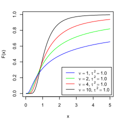
Parameters	${\displaystyle \nu >0\,}$ ${\displaystyle \tau ^{2}>0\,}$
Support	${\displaystyle x\in (0,\infty )}$
PDF	${\displaystyle {\frac {(\tau ^{2}\nu /2)^{\nu /2}}{\Gamma (\nu /2)}}~{\frac {\exp \left[{\frac {-\nu \tau ^{2}}{2x}}\right]}{x^{1+\nu /2}}}}$
CDF	${\displaystyle \Gamma \left({\frac {\nu }{2}},{\frac {\tau ^{2}\nu }{2x}}\right)\left/\Gamma \left({\frac {\nu }{2}}\right)\right.}$
Mean	${\displaystyle {\frac {\nu \tau ^{2}}{\nu -2}}}$ for ${\displaystyle \nu >2\,}$
Mode	${\displaystyle {\frac {\nu \tau ^{2}}{\nu +2}}}$
Variance	${\displaystyle {\frac {2\nu ^{2}\tau ^{4}}{(\nu -2)^{2}(\nu -4)}}}$for ${\displaystyle \nu >4\,}$
Skewness	${\displaystyle {\frac {4}{\nu -6}}{\sqrt {2(\nu -4)}}}$for ${\displaystyle \nu >6\,}$
Excess kurtosis	${\displaystyle {\frac {12(5\nu -22)}{(\nu -6)(\nu -8)}}}$for ${\displaystyle \nu >8\,}$
Entropy	${\displaystyle {\frac {\nu }{2}}\!+\!\ln \left({\frac {\tau ^{2}\nu }{2}}\Gamma \left({\frac {\nu }{2}}\right)\right)}$ ${\displaystyle \!-\!\left(1\!+\!{\frac {\nu }{2}}\right)\psi \left({\frac {\nu }{2}}\right)}$
MGF	${\displaystyle {\frac {2}{\Gamma ({\frac {\nu }{2}})}}\left({\frac {-\tau ^{2}\nu t}{2}}\right)^{\!\!{\frac {\nu }{4}}}\!\!K_{\frac {\nu }{2}}\left({\sqrt {-2\tau ^{2}\nu t}}\right)}$
CF	${\displaystyle {\frac {2}{\Gamma ({\frac {\nu }{2}})}}\left({\frac {-i\tau ^{2}\nu t}{2}}\right)^{\!\!{\frac {\nu }{4}}}\!\!K_{\frac {\nu }{2}}\left({\sqrt {-2i\tau ^{2}\nu t}}\right)}$

The scaled inverse chi-squared distribution ${\displaystyle \psi \,{\mbox{inv-}}\chi ^{2}(\nu )}$, where ${\displaystyle \psi }$ is the scale parameter, equals the univariate inverse Wishart distribution ${\displaystyle {\mathcal {W}}^{-1}(\psi ,\nu )}$ with degrees of freedom ${\displaystyle \nu }$.

This family of scaled inverse chi-squared distributions is linked to the inverse-chi-squared distribution and to the chi-squared distribution:

If ${\displaystyle X\sim \psi \,{\mbox{inv-}}\chi ^{2}(\nu )}$ then ${\displaystyle X/\psi \sim {\mbox{inv-}}\chi ^{2}(\nu )}$ as well as ${\displaystyle \psi /X\sim \chi ^{2}(\nu )}$ and ${\displaystyle 1/X\sim \psi ^{-1}\chi ^{2}(\nu )}$.

Instead of ${\displaystyle \psi }$, the scaled inverse chi-squared distribution is however most frequently parametrized by the scale parameter ${\displaystyle \tau ^{2}=\psi /\nu }$ and the distribution ${\displaystyle \nu \tau ^{2}\,{\mbox{inv-}}\chi ^{2}(\nu )}$ is denoted by ${\displaystyle {\mbox{Scale-inv-}}\chi ^{2}(\nu ,\tau ^{2})}$.

In terms of ${\displaystyle \tau ^{2}}$ the above relations can be written as follows:

If ${\displaystyle X\sim {\mbox{Scale-inv-}}\chi ^{2}(\nu ,\tau ^{2})}$ then ${\displaystyle {\frac {X}{\nu \tau ^{2}}}\sim {\mbox{inv-}}\chi ^{2}(\nu )}$ as well as ${\displaystyle {\frac {\nu \tau ^{2}}{X}}\sim \chi ^{2}(\nu )}$ and ${\displaystyle 1/X\sim {\frac {1}{\nu \tau ^{2}}}\chi ^{2}(\nu )}$.

This family of scaled inverse chi-squared distributions is a reparametrization of the inverse-gamma distribution.

Specifically, if

${\displaystyle X\sim \psi \,{\mbox{inv-}}\chi ^{2}(\nu )={\mbox{Scale-inv-}}\chi ^{2}(\nu ,\tau ^{2})}$   then   ${\displaystyle X\sim {\textrm {Inv-Gamma}}\left({\frac {\nu }{2}},{\frac {\psi }{2}}\right)={\textrm {Inv-Gamma}}\left({\frac {\nu }{2}},{\frac {\nu \tau ^{2}}{2}}\right)}$

Either form may be used to represent the maximum entropy distribution for a fixed first inverse moment ${\displaystyle (E(1/X))}$ and first logarithmic moment ${\displaystyle (E(\ln(X))}$.

The scaled inverse chi-squared distribution also has a particular use in Bayesian statistics. Specifically, the scaled inverse chi-squared distribution can be used as a conjugate prior for the variance parameter of a normal distribution. The same prior in alternative parametrization is given by the inverse-gamma distribution.

Characterization

The probability density function of the scaled inverse chi-squared distribution extends over the domain ${\displaystyle x>0}$ and is

${\displaystyle f(x;\nu ,\tau ^{2})={\frac {(\tau ^{2}\nu /2)^{\nu /2}}{\Gamma (\nu /2)}}~{\frac {\exp \left[{\frac {-\nu \tau ^{2}}{2x}}\right]}{x^{1+\nu /2}}}}$

where ${\displaystyle \nu }$ is the degrees of freedom parameter and ${\displaystyle \tau ^{2}}$ is the scale parameter. The cumulative distribution function is

${\displaystyle F(x;\nu ,\tau ^{2})=\Gamma \left({\frac {\nu }{2}},{\frac {\tau ^{2}\nu }{2x}}\right)\left/\Gamma \left({\frac {\nu }{2}}\right)\right.}$

${\displaystyle =Q\left({\frac {\nu }{2}},{\frac {\tau ^{2}\nu }{2x}}\right)}$

where ${\displaystyle \Gamma (a,x)}$ is the incomplete gamma function, ${\displaystyle \Gamma (x)}$ is the gamma function and ${\displaystyle Q(a,x)}$ is a regularized gamma function. The characteristic function is

${\displaystyle \varphi (t;\nu ,\tau ^{2})=}$

${\displaystyle {\frac {2}{\Gamma ({\frac {\nu }{2}})}}\left({\frac {-i\tau ^{2}\nu t}{2}}\right)^{\!\!{\frac {\nu }{4}}}\!\!K_{\frac {\nu }{2}}\left({\sqrt {-2i\tau ^{2}\nu t}}\right),}$

where ${\displaystyle K_{\frac {\nu }{2}}(z)}$ is the modified Bessel function of the second kind.

Parameter estimation

The maximum likelihood estimate of ${\displaystyle \tau ^{2}}$ is

${\displaystyle \tau ^{2}=n/\sum _{i=1}^{n}{\frac {1}{x_{i}}}.}$

The maximum likelihood estimate of ${\displaystyle {\frac {\nu }{2}}}$ can be found using Newton's method on:

${\displaystyle \ln \left({\frac {\nu }{2}}\right)-\psi \left({\frac {\nu }{2}}\right)={\frac {1}{n}}\sum _{i=1}^{n}\ln \left(x_{i}\right)-\ln \left(\tau ^{2}\right),}$

where ${\displaystyle \psi (x)}$ is the digamma function. An initial estimate can be found by taking the formula for mean and solving it for ${\displaystyle \nu .}$ Let ${\displaystyle {\bar {x}}={\frac {1}{n}}\sum _{i=1}^{n}x_{i}}$ be the sample mean. Then an initial estimate for ${\displaystyle \nu }$ is given by:

${\displaystyle {\frac {\nu }{2}}={\frac {\bar {x}}{{\bar {x}}-\tau ^{2}}}.}$

Bayesian estimation of the variance of a normal distribution

The scaled inverse chi-squared distribution has a second important application, in the Bayesian estimation of the variance of a Normal distribution.

According to Bayes' theorem, the posterior probability distribution for quantities of interest is proportional to the product of a prior distribution for the quantities and a likelihood function:

${\displaystyle p(\sigma ^{2}|D,I)\propto p(\sigma ^{2}|I)\;p(D|\sigma ^{2})}$

where D represents the data and I represents any initial information about σ² that we may already have.

The simplest scenario arises if the mean μ is already known; or, alternatively, if it is the conditional distribution of σ² that is sought, for a particular assumed value of μ.

Then the likelihood term L(σ²|D) = p(D|σ²) has the familiar form

${\displaystyle {\mathcal {L}}(\sigma ^{2}|D,\mu )={\frac {1}{\left({\sqrt {2\pi }}\sigma \right)^{n}}}\;\exp \left[-{\frac {\sum _{i}^{n}(x_{i}-\mu )^{2}}{2\sigma ^{2}}}\right]}$

Combining this with the rescaling-invariant prior p(σ²|I) = 1/σ², which can be argued (e.g. following Jeffreys) to be the least informative possible prior for σ² in this problem, gives a combined posterior probability

${\displaystyle p(\sigma ^{2}|D,I,\mu )\propto {\frac {1}{\sigma ^{n+2}}}\;\exp \left[-{\frac {\sum _{i}^{n}(x_{i}-\mu )^{2}}{2\sigma ^{2}}}\right]}$

This form can be recognised as that of a scaled inverse chi-squared distribution, with parameters ν = n and τ² = s² = (1/n) Σ (x_i-μ)²

Gelman et al remark that the re-appearance of this distribution, previously seen in a sampling context, may seem remarkable; but given the choice of prior the "result is not surprising".^[1]

In particular, the choice of a rescaling-invariant prior for σ² has the result that the probability for the ratio of σ² / s² has the same form (independent of the conditioning variable) when conditioned on s² as when conditioned on σ²:

${\displaystyle p({\tfrac {\sigma ^{2}}{s^{2}}}|s^{2})=p({\tfrac {\sigma ^{2}}{s^{2}}}|\sigma ^{2})}$

In the sampling-theory case, conditioned on σ², the probability distribution for (1/s²) is a scaled inverse chi-squared distribution; and so the probability distribution for σ² conditioned on s², given a scale-agnostic prior, is also a scaled inverse chi-squared distribution.

Use as an informative prior

If more is known about the possible values of σ², a distribution from the scaled inverse chi-squared family, such as Scale-inv-χ²(n₀, s₀²) can be a convenient form to represent a more informative prior for σ², as if from the result of n₀ previous observations (though n₀ need not necessarily be a whole number):

${\displaystyle p(\sigma ^{2}|I^{\prime },\mu )\propto {\frac {1}{\sigma ^{n_{0}+2}}}\;\exp \left[-{\frac {n_{0}s_{0}^{2}}{2\sigma ^{2}}}\right]}$

Such a prior would lead to the posterior distribution

${\displaystyle p(\sigma ^{2}|D,I^{\prime },\mu )\propto {\frac {1}{\sigma ^{n+n_{0}+2}}}\;\exp \left[-{\frac {ns^{2}+n_{0}s_{0}^{2}}{2\sigma ^{2}}}\right]}$

which is itself a scaled inverse chi-squared distribution. The scaled inverse chi-squared distributions are thus a convenient conjugate prior family for σ² estimation.

Estimation of variance when mean is unknown

If the mean is not known, the most uninformative prior that can be taken for it is arguably the translation-invariant prior p(μ|I) ∝ const., which gives the following joint posterior distribution for μ and σ²,

${\displaystyle {\begin{aligned}p(\mu ,\sigma ^{2}\mid D,I)&\propto {\frac {1}{\sigma ^{n+2}}}\exp \left[-{\frac {\sum _{i}^{n}(x_{i}-\mu )^{2}}{2\sigma ^{2}}}\right]\\&={\frac {1}{\sigma ^{n+2}}}\exp \left[-{\frac {\sum _{i}^{n}(x_{i}-{\bar {x}})^{2}}{2\sigma ^{2}}}\right]\exp \left[-{\frac {n(\mu -{\bar {x}})^{2}}{2\sigma ^{2}}}\right]\end{aligned}}}$

The marginal posterior distribution for σ² is obtained from the joint posterior distribution by integrating out over μ,

${\displaystyle {\begin{aligned}p(\sigma ^{2}|D,I)\;\propto \;&{\frac {1}{\sigma ^{n+2}}}\;\exp \left[-{\frac {\sum _{i}^{n}(x_{i}-{\bar {x}})^{2}}{2\sigma ^{2}}}\right]\;\int _{-\infty }^{\infty }\exp \left[-{\frac {n(\mu -{\bar {x}})^{2}}{2\sigma ^{2}}}\right]d\mu \\=\;&{\frac {1}{\sigma ^{n+2}}}\;\exp \left[-{\frac {\sum _{i}^{n}(x_{i}-{\bar {x}})^{2}}{2\sigma ^{2}}}\right]\;{\sqrt {2\pi \sigma ^{2}/n}}\\\propto \;&(\sigma ^{2})^{-(n+1)/2}\;\exp \left[-{\frac {(n-1)s^{2}}{2\sigma ^{2}}}\right]\end{aligned}}}$

This is again a scaled inverse chi-squared distribution, with parameters ${\displaystyle \scriptstyle {n-1}\;}$ and ${\displaystyle \scriptstyle {s^{2}=\sum (x_{i}-{\bar {x}})^{2}/(n-1)}}$.

Related distributions

• If ${\displaystyle X\sim {\mbox{Scale-inv-}}\chi ^{2}(\nu ,\tau ^{2})}$ then ${\displaystyle kX\sim {\mbox{Scale-inv-}}\chi ^{2}(\nu ,k\tau ^{2})\,}$
• If ${\displaystyle X\sim {\mbox{inv-}}\chi ^{2}(\nu )\,}$ (Inverse-chi-squared distribution) then ${\displaystyle X\sim {\mbox{Scale-inv-}}\chi ^{2}(\nu ,1/\nu )\,}$
• If ${\displaystyle X\sim {\mbox{Scale-inv-}}\chi ^{2}(\nu ,\tau ^{2})}$ then ${\displaystyle {\frac {X}{\tau ^{2}\nu }}\sim {\mbox{inv-}}\chi ^{2}(\nu )\,}$ (Inverse-chi-squared distribution)
• If ${\displaystyle X\sim {\mbox{Scale-inv-}}\chi ^{2}(\nu ,\tau ^{2})}$ then ${\displaystyle X\sim {\textrm {Inv-Gamma}}\left({\frac {\nu }{2}},{\frac {\nu \tau ^{2}}{2}}\right)}$ (Inverse-gamma distribution)
• Scaled inverse chi square distribution is a special case of type 5 Pearson distribution

References

• Gelman A. et al (1995), Bayesian Data Analysis, pp 474–475; also pp 47, 480